mouse_alzheimer

Last updated: 2020-07-03

Checks: 6 0

Knit directory: SecretUtils/

This reproducible R Markdown analysis was created with workflowr (version 1.3.0). The Checks tab describes the reproducibility checks that were applied when the results were created. The Past versions tab lists the development history.

R Markdown file: up-to-date

Great! Since the R Markdown file has been committed to the Git repository, you know the exact version of the code that produced these results.

Environment: empty

Great job! The global environment was empty. Objects defined in the global environment can affect the analysis in your R Markdown file in unknown ways. For reproduciblity it’s best to always run the code in an empty environment.

Seed: set.seed(20190415)

The command set.seed(20190415) was run prior to running the code in the R Markdown file. Setting a seed ensures that any results that rely on randomness, e.g. subsampling or permutations, are reproducible.

Session information: recorded

Great job! Recording the operating system, R version, and package versions is critical for reproducibility.

Cache: none

Nice! There were no cached chunks for this analysis, so you can be confident that you successfully produced the results during this run.

Repository version: b7acbc7

Great! You are using Git for version control. Tracking code development and connecting the code version to the results is critical for reproducibility. The version displayed above was the version of the Git repository at the time these results were generated.

Note that you need to be careful to ensure that all relevant files for the analysis have been committed to Git prior to generating the results (you can use wflow_publish or wflow_git_commit). workflowr only checks the R Markdown file, but you know if there are other scripts or data files that it depends on. Below is the status of the Git repository when the results were generated:


Ignored files:
    Ignored:    .Rhistory
    Ignored:    .Rproj.user/

Untracked files:
    Untracked:  .Rbuildignore
    Untracked:  R/asdf_bk
    Untracked:  R/hello.R
    Untracked:  R_bk/
    Untracked:  analysis/eps_joint_all.bmp
    Untracked:  analysis/grid_of_grids.pdf
    Untracked:  analysis/make_scanpy_viktor.R
    Untracked:  analysis/morphine.Rmd
    Untracked:  analysis/mouse_alzheimer_annotating.Rmd
    Untracked:  analysis/mouse_alzheimer_preproc.Rmd
    Untracked:  analysis/paga.Rmd
    Untracked:  analysis/paga3.Rmd
    Untracked:  analysis/pca_dependency.Rmd
    Untracked:  analysis/simulate_data.Rmd
    Untracked:  analysis/simulate_data2.Rmd
    Untracked:  analysis/simulate_data3.Rmd
    Untracked:  analysis/simulations_plots3_bk.Rmd
    Untracked:  analysis/simulations_plots4.Rmd
    Untracked:  analysis/simulations_plots5_bk.Rmd
    Untracked:  analysis/simulations_plots6.Rmd
    Untracked:  analysis/subtype_distances.Rmd
    Untracked:  analysis/subtype_distances2.Rmd
    Untracked:  analysis/subtype_distances4.Rmd
    Untracked:  analysis/subtype_distances_redux.Rmd
    Untracked:  analysis/subtype_distances_revenge.Rmd
    Untracked:  analysis/test_output.Rmd
    Untracked:  analysis/transmute_peters_code.Rmd
    Untracked:  docs/figure/paga.Rmd/
    Untracked:  man/

Unstaged changes:
    Modified:   R/asdf.R
    Modified:   analysis/correlation_stuff.Rmd
    Modified:   analysis/jensen_shannon_stuff.Rmd
    Modified:   analysis/misc_metrics.Rmd
    Modified:   analysis/paga2.Rmd
    Modified:   analysis/paga_analyses.Rmd
    Modified:   analysis/pancreas_indrop.Rmd
    Modified:   analysis/sanity_check.Rmd
    Modified:   analysis/simulations_plots.Rmd
    Modified:   analysis/simulations_plots3.Rmd
    Modified:   analysis/simulations_plots5.Rmd
    Modified:   analysis/simulations_plots_intro.Rmd
    Modified:   analysis/subtype_distances3.Rmd
    Modified:   analysis/transmute_code_eps.Rmd
    Modified:   analysis/transmute_code_eps_2.Rmd
    Modified:   analysis/visualizations.Rmd

Note that any generated files, e.g. HTML, png, CSS, etc., are not included in this status report because it is ok for generated content to have uncommitted changes.

These are the previous versions of the R Markdown and HTML files. If you’ve configured a remote Git repository (see ?wflow_git_remote), click on the hyperlinks in the table below to view them.

File	Version	Author	Date	Message
Rmd	b7acbc7	githubz0r	2020-07-03	update the script a bit
html	0c4c367	githubz0r	2019-06-06	Build site.
Rmd	056d849	githubz0r	2019-06-06	some new plots

Load conos, pagoda2 and SecretUtils etc.

library(conos)
library(tidyverse)
devtools::load_all('/home/larsc/SecretUtils')
require(pagoda2)
library(pheatmap)
library(irlba)
library(igraph)
mouse_annot <- read.csv(file.path('/home/larsc/data/mouse_alzheimer/mouse_alzheimers_annotation_filtered_subtypes.csv'))
mouse_annot$subtype_condition <- paste0(mouse_annot$celltype, '.', mouse_annot$condition)

load conos object

mouse_con <- readRDS('/home/larsc/data/mouse_alzheimer/mouse_alzheimers_conos_procced_graphed.rds')

Rbind panels from conos objects

rbound_panel <- RbindPanel(mouse_con)
# sorting it just in case
rbound_panel <- rbound_panel[order(rbound_panel %>% rownames),]

Make groups for colorful tsne plots of the dataset

nr_annot <- setNames(mouse_annot$mouse_nr, mouse_annot$Well_ID)
batch_annot <- setNames(mouse_annot$Amp_batch_ID, mouse_annot$Well_ID)
condition_annot <- setNames(mouse_annot$condition, mouse_annot$Well_ID)
celltype_annot <- setNames(mouse_annot$celltype, mouse_annot$Well_ID)
sub_cond_annot <- setNames(mouse_annot$subtype_condition, mouse_annot$Well_ID)

table(nr_annot)

nr_annot
AD6m_mouse1 AD6m_mouse2 AD6m_mouse3 WT6m_mouse1 WT6m_mouse2 WT6m_mouse3 
       1517        2264        2264        1514        2651        2273

table(celltype_annot)

celltype_annot
         Bcells    granulocytes       microglia PvascMacro+Mono 
            723             446           10018             469 
      T+NKcells 
            827

Plot graph with different annotations

mouse_con$plotGraph(groups=condition_annot, font.size=3, size=0.3, alpha=0.3, show.legend=T)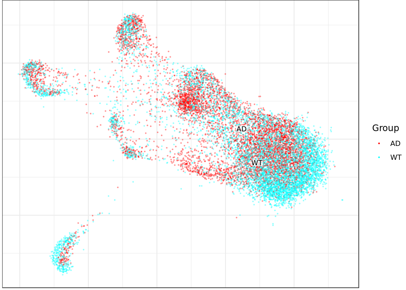

Version	Author	Date
0c4c367	githubz0r	2019-06-06

mouse_con$plotGraph(groups=celltype_annot, font.size=3, size=0.3, alpha=0.3, show.legend=T)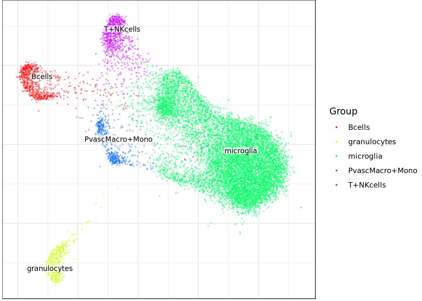

Version	Author	Date
0c4c367	githubz0r	2019-06-06

mouse_con$plotGraph(groups=sub_cond_annot, font.size=3, size=0.3, alpha=0.3, show.legend=T)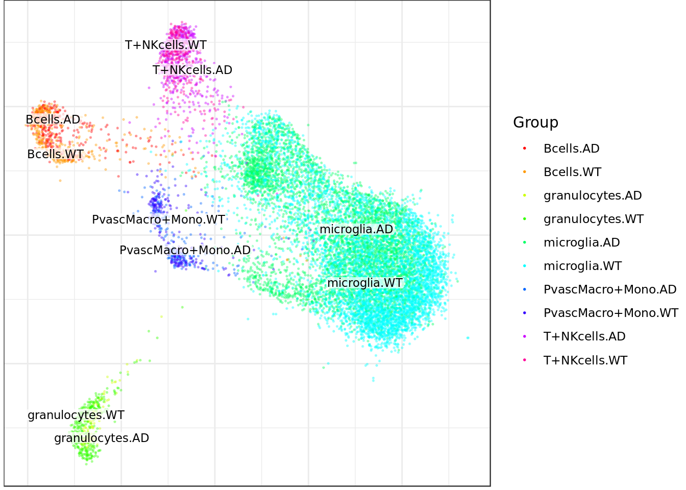

Version	Author	Date
0c4c367	githubz0r	2019-06-06

mouse_con$plotGraph(groups=nr_annot, font.size=3, size=0.3, alpha=0.3, show.legend=T)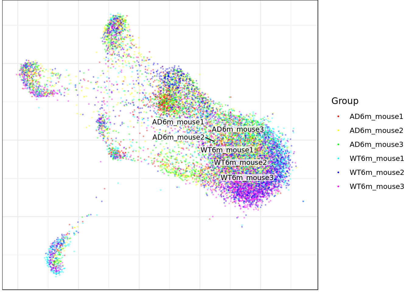

Version	Author	Date
0c4c367	githubz0r	2019-06-06

Initiate some variables

od_genes = conos:::getOdGenesUniformly(mouse_con$samples, 3000)
state_split <- split(mouse_annot, mouse_annot$condition, drop=TRUE)
subtype_split <- state_split %>% lapply(function(x){split(x, x$celltype, drop=TRUE)})

Jensen Shannon between AD and WT, overall (microglia has by far the most cells so this will heavily skew the result due to dropout)

sub_mats_probs <- SecretUtils::GetSubMats(rbound_panel, mouse_annot$Well_ID, mouse_annot$celltype, mouse_annot$condition, 
                                          normalize=T, pseudo.prob=10^-8)

all_dists <- Map(JensenShannon, sub_mats_probs$AD, sub_mats_probs$WT) %>% as_tibble
all_dists_gathered <- gather(all_dists, key=subtype, value=js_distance)
ggplot(all_dists_gathered, aes(y=js_distance, x=subtype)) +geom_bar(stat='identity') +
  theme(axis.text.x = element_text(angle = -90, hjust = 1))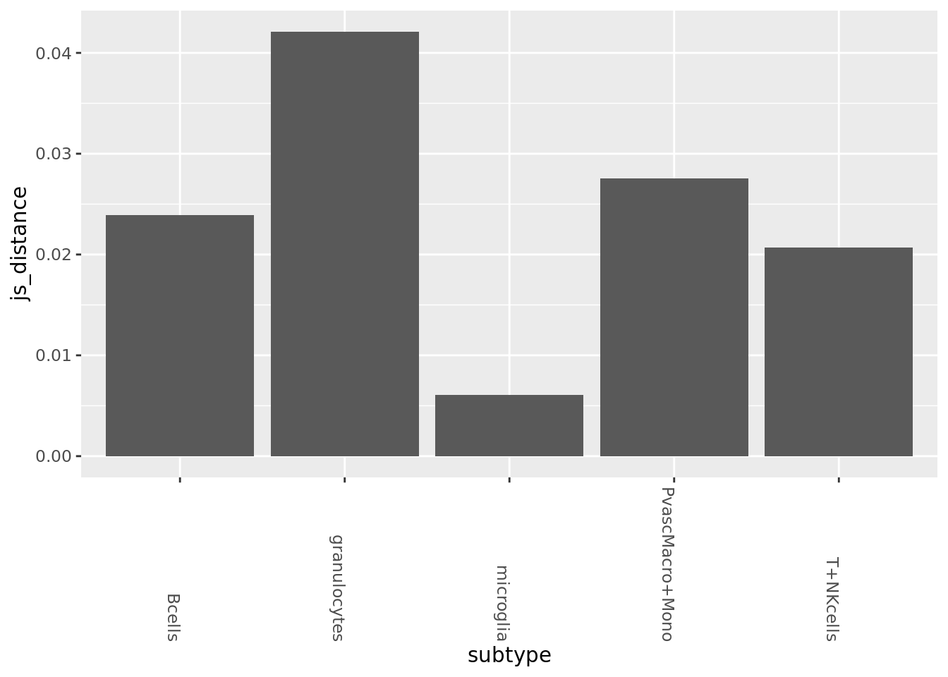

Version	Author	Date
0c4c367	githubz0r	2019-06-06

Violins plots of between condition distances(slightly older function, hence some not ideal practices regarding input variables, but gets the job done).

wtcellprobs <- IndividualCellProbs(state_split$WT, rbound_panel, 1, 7, 100, od_genes, 10^(-8))
adcellprobs <- IndividualCellProbs(state_split$AD, rbound_panel, 1, 7, 100, od_genes, 10^(-8))
all_singlecell_dists <- Map(CalculateAllJSD, wtcellprobs, adcellprobs)
all_sc_dists <- all_singlecell_dists %>% as_tibble
all_scd_gathered <- gather(all_sc_dists, key=subtype, value=jsd)
ggplot(all_scd_gathered, aes(y=jsd, x=subtype)) + geom_violin(aes(col=subtype))+
  theme(axis.text.x = element_text(angle = -90, hjust = 1))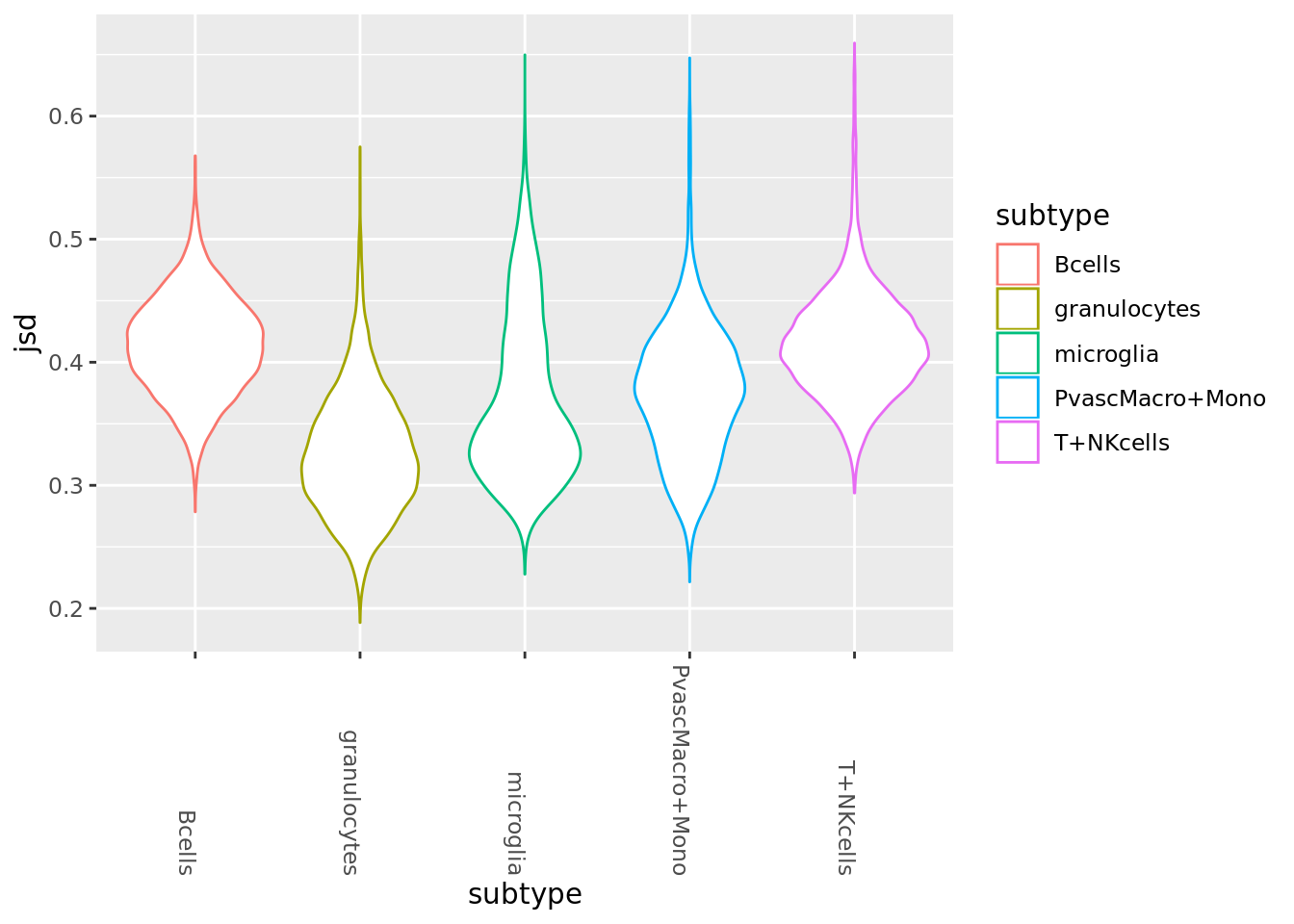

PCA for correlation (correlation is very biased in gene expression space)

pca_cm <- prcomp_irlba(rbound_panel[, od_genes],n=100)
pca_cmat <- pca_cm$x
rownames(pca_cmat) <- rownames(rbound_panel)
pca_genes <- colnames(pca_cmat)

sub_mats_pca <- SecretUtils::GetSubMats(pca_cmat, mouse_annot$Well_ID, mouse_annot$celltype, mouse_annot$condition)

all_dists <- Map(function(x,y){1-cor(x,y)}, sub_mats_pca$AD, sub_mats_pca$WT) %>% as_tibble
all_dists_gathered <- gather(all_dists, key=subtype, value=correlation.distance)
ggplot(all_dists_gathered, aes(y=correlation.distance, x=subtype)) +geom_bar(stat='identity') +
  theme(axis.text.x = element_text(angle = -90, hjust = 1))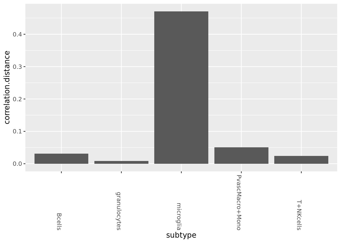

Version	Author	Date
0c4c367	githubz0r	2019-06-06

Plot showing which fractions belong to which celltype for the corresponding conditions.

FractionalPlot(mouse_annot$mouse_nr, mouse_annot$celltype, mouse_annot$condition)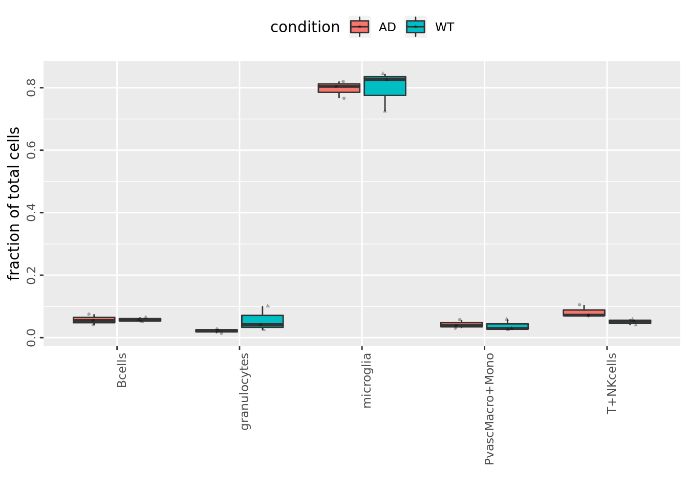

PAGA using unaligned graph (KNN graph where edges are correlation distance in PCA space). Small value = less connected, i.e. a similarity metric, not distance. Note that in general we do not trust the PAGA metric as unbiased, see the simulation plots.

raw_mouse <- RbindRaw(mouse_con)
mouse_unaligned_adj <- GenerateUnalignedAdj(raw_mouse, cellid.vector=mouse_annot$Well_ID)[mouse_annot$Well_ID, mouse_annot$Well_ID]

12483 cells, 34016 genes; normalizing ... using plain model winsorizing ... log scale ... done.
calculating variance fit ... using gam 134 overdispersed genes ... 134 persisting ... done.
running PCA using 3000 OD genes .... done

subtype_order <- (paste0(mouse_annot$celltype) %>% unique)[order(paste0(mouse_annot$celltype) %>% unique)]
membership_vec <- as.numeric(factor(mouse_annot$subtype_condition))

connectivities <- GetPagaMatrix(mouse_unaligned_adj, membership_vec, scale=F)
linearized_stats <- seq(1, dim(connectivities)[1], 2) %>% sapply(function(i){connectivities[i,i+1]})

paga_df <- bind_cols(value=linearized_stats, subtype=subtype_order)
ggplot(paga_df, aes(y=linearized_stats, x=subtype)) +geom_point()+
  theme(axis.text.x = element_text(angle = -90, hjust = 1))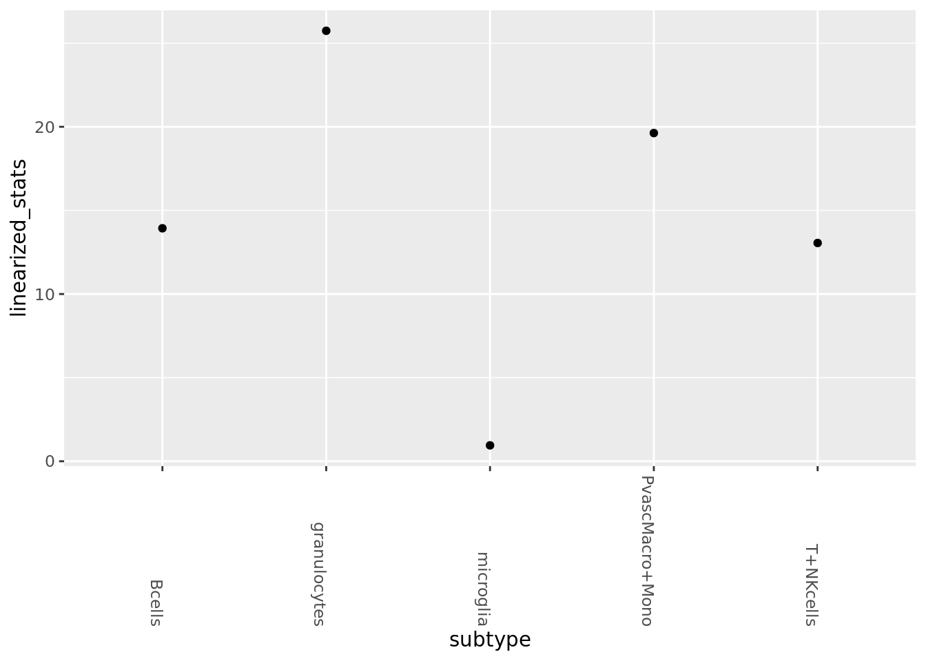

sessionInfo()

R version 3.5.3 (2019-03-11)
Platform: x86_64-pc-linux-gnu (64-bit)
Running under: Ubuntu 18.04.2 LTS

Matrix products: default
BLAS: /usr/lib/x86_64-linux-gnu/atlas/libblas.so.3.10.3
LAPACK: /usr/lib/x86_64-linux-gnu/atlas/liblapack.so.3.10.3

locale:
 [1] LC_CTYPE=en_US.UTF-8       LC_NUMERIC=C              
 [3] LC_TIME=en_US.UTF-8        LC_COLLATE=en_US.UTF-8    
 [5] LC_MONETARY=en_US.UTF-8    LC_MESSAGES=en_US.UTF-8   
 [7] LC_PAPER=en_US.UTF-8       LC_NAME=C                 
 [9] LC_ADDRESS=C               LC_TELEPHONE=C            
[11] LC_MEASUREMENT=en_US.UTF-8 LC_IDENTIFICATION=C       

attached base packages:
[1] stats     graphics  grDevices utils     datasets  methods   base     

other attached packages:
 [1] irlba_2.3.3       pheatmap_1.0.12   pagoda2_0.1.0    
 [4] SecretUtils_0.1.0 reshape2_1.4.3    magrittr_1.5     
 [7] forcats_0.4.0     stringr_1.4.0     dplyr_0.8.3      
[10] purrr_0.3.2       readr_1.3.1       tidyr_0.8.3      
[13] tibble_2.1.3      ggplot2_3.2.0     tidyverse_1.2.1  
[16] conos_1.0.0       igraph_1.2.4.1    Matrix_1.2-17    

loaded via a namespace (and not attached):
 [1] nlme_3.1-139       matrixStats_0.54.0 fs_1.3.1          
 [4] usethis_1.5.0      lubridate_1.7.4    devtools_2.0.2    
 [7] RColorBrewer_1.1-2 httr_1.4.0         rprojroot_1.3-2   
[10] tools_3.5.3        backports_1.1.4    R6_2.4.0          
[13] mgcv_1.8-28        lazyeval_0.2.2     colorspace_1.4-1  
[16] withr_2.1.2        tidyselect_0.2.5   gridExtra_2.3     
[19] prettyunits_1.0.2  processx_3.3.1     compiler_3.5.3    
[22] git2r_0.25.2       cli_1.1.0          rvest_0.3.4       
[25] xml2_1.2.0         desc_1.2.0         labeling_0.3      
[28] triebeard_0.3.0    scales_1.0.0       callr_3.2.0       
[31] pbapply_1.4-0      digest_0.6.20      rmarkdown_1.12    
[34] base64enc_0.1-3    pkgconfig_2.0.2    htmltools_0.3.6   
[37] sessioninfo_1.1.1  rlang_0.4.0        readxl_1.3.1      
[40] rstudioapi_0.10    shiny_1.3.2        generics_0.0.2    
[43] jsonlite_1.6       dendextend_1.12.0  Rcpp_1.0.1        
[46] munsell_0.5.0      abind_1.4-5        viridis_0.5.1     
[49] stringi_1.4.3      whisker_0.3-2      yaml_2.2.0        
[52] MASS_7.3-51.3      pkgbuild_1.0.3     Rtsne_0.15        
[55] plyr_1.8.4         grid_3.5.3         ggrepel_0.8.1     
[58] parallel_3.5.3     promises_1.0.1     crayon_1.3.4      
[61] lattice_0.20-38    splines_3.5.3      haven_2.1.0       
[64] cowplot_0.9.4      hms_0.4.2          knitr_1.22        
[67] ps_1.3.0           pillar_1.4.2       rjson_0.2.20      
[70] pkgload_1.0.2      glue_1.3.1         evaluate_0.13     
[73] data.table_1.12.2  remotes_2.0.4      modelr_0.1.4      
[76] urltools_1.7.3     httpuv_1.5.1       testthat_2.1.1    
[79] cellranger_1.1.0   gtable_0.3.0       assertthat_0.2.1  
[82] xfun_0.6           mime_0.6           xtable_1.8-4      
[85] broom_0.5.2        later_0.8.0        viridisLite_0.3.0 
[88] memoise_1.1.0      Rook_1.1-1         workflowr_1.3.0   
[91] brew_1.0-6

mouse_alzheimer_analysis

githubz0r

2019-06-6